Help Topics

Input Fields
Advanced Input Fields
Output
MultiFoXS

Input Fields

FoXS requires only one mandatory input parameter, the input molecule:

• Input Molecule: A user has to specify PDB id and chain of the molecule (pdb:chain, e.g. 1ukr:A) or upload a file containing the structure of the molecule in PDB or mmCIF format.

  It is also possible to upload a zip file with several PDB or mmCIF structures. In this case each structure will be fitted to the profile separately. Only zip compression is currently supported. Note that profile calculation is performed for up to 100 PDB/mmCIF files. If you need more extensive profile evaluations please use download version.

  For NMR structures please select suitable MODEL reading option from advanced parameters.

  Please use standard PDB atom naming in the files you upload!

  Hydrogen atoms for proteins and nucleic acids are considered implicitly by adding their form factors to those for their bound heavy atom. If your structure includes other groups, such as lipids, sugars etc., we recommend adding all the hydrogens and turning off "implicit hydrogens" option of FoXS to achieve higher accuracy. Hydrogen atoms can be added with Reduce.

  IMPORTANT!
  Please make sure there are no missing residues/nucleic acids in the structure you upload!
  Your structure should be as close as possible to the sample you used to collect the experimental data!
  It is highly recommended to model missing loops, disordered N- and C- termini and His tags.

• Experimental profile: A user can upload a file with experimental profile (optional). In this case the theoretical profile will be fitted to the experimental one. The experimental file should have 3 columns: q, I(q) and error:

  # q intensity error
  0.00000 3280247.73 1904.037
  0.00060 3280164.59 1417.031
  0.00120 3279915.19 1840.032
  0.00180 3279499.57 1566.084

  Header lines should be preceded by #.

  Please note that: q = (4π sin θ) / λ,
  where 2θ is the scattering angle and λ is the wavelength of the incident X-ray beam.

  Sample input file for lysozyme (PDB code 6lyz) can be found here.
  If your experimental profile does not contain an error column, the server will add 5% error with Poisson distribution.

• e-mail address: An e-mail address for receiving the link to the results page (optional). The results page will be available for at least a week.
• Job name: The job can be assigned an (optional) name to help organize multiple results pages.

Advanced Input Fields

Setting these parameters is optional:

• Maximal q value The theoretical profile will be computed up till this q value (default = 0.5)
• Profile size Number of discrete points that represent the profile (default = 500)
• Hydration Layer Set hydration layer parameter c₂
• Excluded volume Set excluded volume parameter c₁
• Implicit hydrogens Consider hydrogens implicitly
• Residue level computation Perform coarse grained profile computation for Ca atoms only. This is not as accurate as full atom calculation, can be used only for large structures
• Background Adjustment This option applies background adjustment to the input experimental profile. As a result the profile is corrected at higher q values, the intensity values are decreased (see Ciccariello et al. (1988) for details)
• Offset Use constant offset in profile fitting
• MODEL reading FoXS supports all possible options of handling PDB files with MODEL records. By default MODEL records are ignored and all ATOM records are read into a single structure. Alternatively it is possible to read in the first MODEL only or all the MODELs into separate structures. Multi-model mmCIF files (where models are distinguished by atom_site.pdbx_PDB_model_num) are handled similarly; by default the model number is ignored, but the user can choose to read only atoms from atom_site with the first model number, or to read a separate structure for each unique model number.
• Experimental profile units FoXS supports input profiles with q in 1/Å and 1/nm. By default the units of the input profile are determined automatically. Alternatively, the user can set the units.

Output

• Input PDB (or Input mmCIF)
• Input profile
• FoXS output

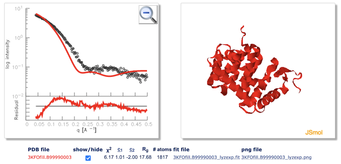
The server displays the profile fit along with the residuals ((experimental-computed)/error) on the left side of the window. The input structure is displayed in a JSmol window. The input experimental profile is shown with black dots, while the theoretical profile is a red line. The user can zoom on different parts of the fit plot, rotate the structure in the JSmol window, and use show/hide button to display or hide the computed profile and the corresponding structure. The file with the theoretical profile fitted to the experimental one can be downloaded using the link under the plot. The format of the fit file is the same as the input profile files, with additional column added that included the calculated profile.

The quality of the fit, χ² value, is printed below the plot.

There are 2 free parameters in profile fitting:

(i) c₁ - is the scaling of the atomic radius and it controls the exluded volume of the molecule
The default value is c₁ = 1.0. During fitting, we allow up to 1% decrease in the radius and up to 5% increase (0.99 ≤ c₁ ≤ 1.05).

(ii) c₂ - is used to adjust the difference between the densities of the hydration layer and the bulk water. This parameter controls the density of the water layer around the molecule.

The default value is c₂ = 0.0. During fitting, the value of c₂ can vary from 0 to 4.0, reflecting an estimate of up to four water molecule neighbors for an exposed solute atom. This threshold is comparable to the average number of water molecules within 3Å of each other in the TIP3P water box. The hydration shell density for c₂ = 4.0 is 0.388e/ų.

The density of the hydration layer around the protein can, in principle, be lower than that of bulk water, depending on the amount of surface charge. Therefore, we also allow c₂ to be slightly negative (-2.0 ≤ c₂ ≤ 4.0). The hydration shell density for c₂ = -2.0 is 0.307e/ų.

Given experimental profile, FoXS finds a combination of c₁ and c₂ that achieves the best fit (lowest χ² value) to the experimental data.

IMPORTANT!
Extreme values of c₁ and c₂ parameters often indicate data overfitting. For example, if you have missing residues in the structure, FoXS can compensate for the missing electron density by increasing the hydration layer density by setting c₂ parameter to the maximal value of 4.0. These values are flagged by FoXS in the results table to alert the users of possible overfitting.

MultiFoXS

The unique capability of FoXS webserver is a possibility to account for multiple states contributing to a single observed SAXS profile. Multiple states can correspond to conformational heterogeneity (multiple conformations of the same protein or complex) and/or compositional heterogeneity (varying contents of protein and ligand molecules in the system).

If multiple PDB or mmCIF files were uploaded by the user, in addition to profile calculation for each structure, the server will also run enumeration and fitting of multiple structures to the input profile. Here is an example.